Ansys CFD
Convergence is a common issue in Computational Fluid Dynamics (CFD). Many engineers face problems while running simulations in Ansys CFD. If a solution does not converge, the results may be incorrect. This blog explains how to fix convergence issues in Ansys CFD simulations. It is meant for learners, students, and professionals seeking practical solutions.
What is Convergence in Ansys CFD?
Imagine you’re trying to find the exact center of a moving target by repeatedly throwing darts. With each throw, your darts get closer and closer to the center. In a CFD simulation, convergence is similar. The solver repeatedly calculates values for things like velocity, pressure, and temperature across a mesh (a network of small cells that represent your model). With each iteration (like each dart throw), these calculated values should get closer to a stable, unchanging solution.
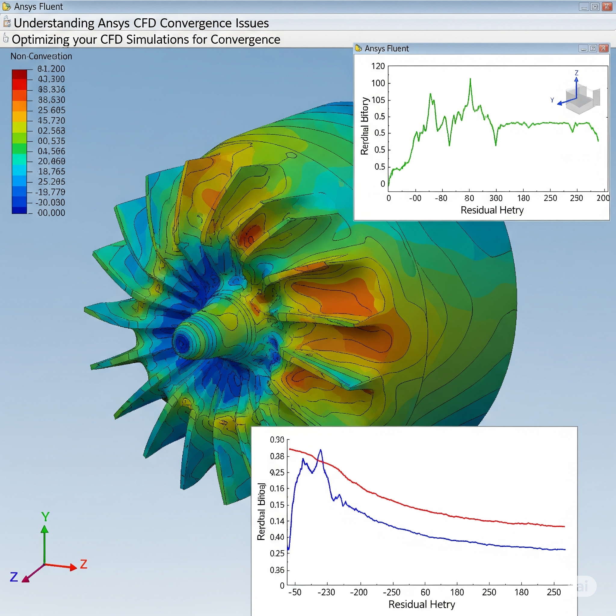
We typically track convergence by looking at residuals in Ansys Fluent. Residuals are essentially measures of how “unbalanced” the equations are at each point in the mesh. As the simulation progresses, these residuals should decrease over many orders of magnitude, ideally reaching very small values (e.g., 10−3 to 10−6 for most flow variables). When they stop changing significantly and stay below a certain threshold, we say the simulation has converged. This threshold is known as the convergence criteria in Ansys
Why Do Ansys Fluent Not Converge?
Several factors can cause a simulation to encounter solver divergence or CFD simulation errors, leading to Ansys Fluent convergence problems. Understanding these causes is the first step to how to solve convergence error in Ansys CFD.
Poor Mesh Quality: The mesh is the foundation of any CFD simulation. If the mesh has highly distorted cells, very large aspect ratios (cells that are very long and thin), or sudden changes in cell size, it can introduce numerical stability problems. Think of it like building a house on a shaky foundation; it’s prone to collapse.
Incorrect Boundary Conditions: Boundary conditions tell the solver what’s happening at the edges of your simulation domain (e.g., inlet velocity, outlet pressure, wall temperature). If you set these incorrectly or inconsistently, the solver can struggle to find a stable solution. For example, trying to push too much fluid through a small opening or applying physically impossible temperatures can lead to divergence.
Inappropriate Physics Models: CFD simulations often involve complex physical phenomena like turbulence, heat transfer, and multiphase flow. Using the wrong turbulence model (e.g., trying to use a simple laminar model for a highly turbulent flow) or an unsuitable multiphase model can lead to instability.
Aggressive Solver Settings: The solver uses various numerical schemes and iterative solvers to arrive at a solution. If you use overly aggressive settings, such as very high under-relaxation factors or large time step control (for transient simulations), the solver might overshoot the solution and diverge.
Complex Geometries: Very intricate geometries with sharp corners or very small features can pose challenges for meshing and, consequently, for the solver to converge.
Poor Initial Conditions: Sometimes, the initial guess for the flow field can be too far from the actual solution, making it difficult for the solver to start converging smoothly.

Tips to Fix CFD Simulation Not Converging
Don’t despair if your simulation isn’t converging! There are many strategies you can employ to troubleshoot and resolve these issues. Here are some best practices for convergence in Ansys Fluent and how to troubleshoot Ansys CFD simulation errors:
1. Mesh Refinement and Quality Improvement
The mesh is often the culprit.
Check Mesh Quality: In Ansys Meshing or Fluent, use the “Check Mesh” utility. Look for minimum orthogonal quality, maximum aspect ratio, and skewness. Aim for orthogonal quality above 0.1, aspect ratio below 100 (ideally much lower for critical regions), and skewness below 0.85.
Local Refinement: Refine the mesh in areas with high gradients (e.g., near walls, around obstacles, or where flow features are important). This means adding more cells to capture the physics accurately.
Smooth Transitions: Ensure gradual transitions in cell size from fine to coarse regions. Abrupt changes can cause problems.
Use Inflation Layers: For flows with boundary layers (e.g., flow over an airfoil), add inflation layers near walls to capture the steep velocity gradients accurately. This is crucial for accurate drag and lift predictions and can significantly improve convergence.
2. Review and Adjust Boundary Conditions
Incorrect boundary condition setup is a common reason for divergence.
Physical Realism: Ensure your boundary conditions are physically realistic. For example, don’t set a pressure outlet to a value lower than the inlet if there’s no mechanism to reduce pressure in between.
Consistency: Make sure all boundary conditions are consistent with each other. If you have an inlet velocity, ensure the mass flow rate at the outlet is also consistent.
Gradual Application (for Transient Simulations): For transient simulations, you might need to ramp up certain boundary conditions gradually rather than applying them suddenly.
3. Optimize Ansys CFD Solver Settings
Tweaking Ansys CFD solver settings can significantly impact convergence.
Under-Relaxation Factors (URFs): URFs control how much the solution updates with each iteration. Lowering URFs (e.g., from 0.5 to 0.2) makes the solution more stable but also slower to converge. For initial runs, start with lower URFs and gradually increase them once the solution shows signs of stability. You can access these in Fluent under “Solution Control.”
Discretization Schemes: Higher-order discretization schemes (e.g., second-order) are more accurate but can be less stable. If you’re having trouble, try starting with first-order schemes and then switch to higher-order once the solution is stable.
Pressure-Velocity Coupling: For steady-state simulations, choosing the right pressure-velocity coupling scheme is vital. SIMPLE and PISO are common choices. SIMPLE is generally more robust for initial convergence, while PISO can be better for transient or complex flows. Coupled solvers are often faster but require good initial conditions.
Time Step Control (for Transient Simulations): For transient simulations, a small time step is crucial for stability. If your Courant number (CFL) is too high, the simulation will likely diverge. Aim for a CFL number generally less than 1 for explicit schemes and often higher for implicit schemes, but still controlled.
Solver Type: Ansys Fluent offers different iterative solvers (e.g., AMG, F-Cycle). Experiment with different solvers or their settings if one isn’t performing well.
4. Smart Initialization
A good starting point can help the solver find its way.
Hybrid Initialization: Fluent’s hybrid initialization often provides a reasonable initial guess for many flow fields.
Patching: For specific problems, you might need to “patch” initial values into certain regions of the domain, perhaps based on a simpler analytical solution or a previous, converged simulation.
FMG Initialization: For complex flows, Full Multigrid (FMG) initialization can be very effective in generating a good initial flow field.
5. Turbulence Modeling Considerations
Choosing and setting up the turbulence model correctly is vital for turbulent flows.
Model Selection: Select an appropriate turbulence modeling scheme based on your flow. For example, for simple internal flows, k−ϵ or k−ω models might suffice. For flows with separation and complex aerodynamics, SST k−ω often performs better.
Y+ Values: For wall-resolved turbulence models, ensure your mesh provides appropriate Y+ values near walls. Incorrect Y+ can lead to inaccurate results and convergence issues.
6. Monitoring and Debugging Residuals
Plot Residuals: Always monitor your residual plots during the simulation. Look for smooth decay. If residuals flatline at a high value or start increasing, it’s a sign of divergence.
Monitor Quantities of Interest: In addition to residuals, monitor physical quantities like mass flow rate at inlets/outlets, lift/drag coefficients, or temperatures at specific points. When these values become steady, it further indicates convergence.
Continuity Residual: Pay close attention to the continuity residual. High continuity residual often points to mass imbalance issues, which can be related to boundary conditions or mesh quality.
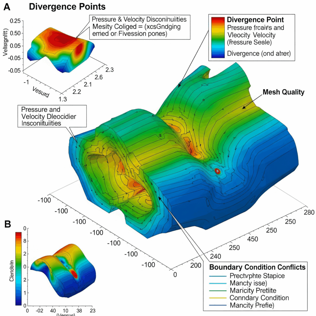
7. Addressing Divergence Points
When a simulation diverges, Fluent often provides clues.
Check for Floating Point Errors: Look for “NaN” (Not a Number) or “Inf” (Infinity) warnings in the console. These indicate numerical instability and often point to severe problems.
Location of Divergence: Sometimes, Fluent will indicate which cell or region is causing the divergence. Investigate that area for mesh quality issues or problematic flow features.
Solution Animation: For transient simulations, creating an animation of the solution can often highlight where and when the divergence starts, helping you pinpoint the cause.
When to Consider Buying Ansys Software
While troubleshooting convergence issues can be part of the learning process, sometimes the problem lies in the complexity of the simulation or the need for advanced features. If you are consistently facing significant challenges with your CFD simulations, or if your projects demand high accuracy and efficiency, it might be time to buy Ansys software with professional support and training. Advanced licenses and modules can offer more robust solvers, meshing tools, and specialized models that can handle even the most challenging fluid dynamics problems.
Conclusion
Fixing convergence issues in Ansys CFD simulations is a common but manageable challenge. By carefully examining your mesh, boundary conditions, solver settings, and turbulence models, you can significantly improve the stability and reliability of your simulations. Remember to start with simpler settings and gradually increase complexity as your simulation shows signs of stability. With patience and a systematic approach, you can overcome these hurdles and achieve accurate, converged results. For advanced solutions and expert guidance, consider reaching out to Corengg Technologies.